Understanding the Tensorflow Quickstart

Note #1: This post will change over time as I better understand what I’m covering here. I’ll leave old text to show the contrasts in understanding.

I will attempt here to establish an ML model, see it do some work, and then break that down and try to understand the work being done as best I can. I will be following this tutorial, the quickstart for tensorflow. And for background on how I got my system set up to be able to do this, check out this post about getting started.

It’s likely I won’t complete this post fully understanding what’s going on here, but that’s OK! Into the unknown, we go!

Note #2: The Jupyter Notebook shows how ‘fast’ it is to get started

The link above ‘about getting started’ gets you to a point where a Jupyter Notebook is open, and inside there is quite a lot of information about what I will cover here. The image below shows some of the topics.

Choose a topic to learn about via tutorials in the jupyter notebook

There are several pre-prepared tutorials in there that have a lot of good information about what the actual task of building a model is. I am by no means trying to replace this set of tutorials, but instead to document my journey through them, and other materials to see what it really took for me to properly understand what a model is, and how to build it.

Enough Preamble, lets go!

Load MNIST dataset?

What is MNIST? It stands for Modified National Institute of Standards and Technology dataset. Here is a link to better describe what that actually is. Short & Sweet, it’s a collection of data that is purpose-built for training and evaluating ML Models. So this is a multi-use tutorial because we’re learning a bit about what it is to load data and set up a model, but then also how to benchmark models, or at least how to prepare a benchmark for models. Cool.

mnist = tf.keras.datasets.mnist

(x_train, y_train), (x_test, y_test) = mnist.load_data()
x_train, x_test = x_train / 255.0, x_test / 255.0

OK so there’s a lot going on here, and I’m very on-off with Python so it takes my brain a second to adjust back to its syntax.

mnist = tf.keras.datasets.mnist 

This is assigning data from the MNIST dataset into a variable. This dataset is a structure with its own methods and properties. I’m not sure what they are all but I know it has at least one method, which we use straight away.

(x_train, y_train), (x_test, y_test) = mnist.load_data()

This line loads the MNIST dataset into four variables: x_train, y_train, x_test, and y_test.

The method load_data(), splits the dataset into training and testing sets, with 60,000 images for training and 10,000 images for testing.

x_train and x_test contain the images themselves, while y_train and y_test contain the corresponding labels (i.e., the correct digit for each image).

x_train, x_test = x_train / 255.0, x_test / 255.0

This line scales the pixel values of the images to be between 0 and 1, which is a common preprocessing step in image classification tasks. I’m not sure of why we need to do that just yet.

But what and where are the pixel values?

Here is what python thinks the x_train variable is:

console output: ~> TensorFlow version: 2.12.0

~> x_train is type: <class 'numpy.ndarray'>

So we know the variables are proper Python classes, from the library NumPy, and they are ndarrays. But what is all that stuff?

NumPy -> a library to provide Python with a way to handle large datasets in a performant
way

ndarray -> the core data structure in NumPy.

From what I’ve read, the arrays and other structures provided in NumPy are implemented in C, so they can be used to implement functionality that is faster than the built-in data structures that Python has.

That would explain why I’ve seen NumPy used in virtually every data project I’ve ever messed with.

Data is Loaded -> Let’s Model

Now comes the part where we start to build a structure that is supposed to produce an output based on our incoming data. Outside of making sure our data is shaped in a predictable way, understanding how to build models is probably the most important part of this whole process. They are what creates the outputs that we find value in. Many of my future posts will be focused on models, but for now let’s keep going with the tutorial.

model = tf.keras.models.Sequential([
  tf.keras.layers.Flatten(input_shape=(28, 28)),
  tf.keras.layers.Dense(128, activation='relu'),
  tf.keras.layers.Dropout(0.2),
  tf.keras.layers.Dense(10)
])

Let’s break this down:

model = tf.keras.models.Sequential([//insert layers here//]):
This line creates a sequential model, which is a linear stack of layers that can be created by passing a list of layers to the constructor. So we are prepping the variable ‘model’ to contain an object that belongs to the keras module.

That object has this type in python: keras.engine.sequential.Sequential object

So it’s not a regular old list, but it’s a ‘series’ set of layers. I don’t quite understand the layers yet. I get that the data passes through them, and the layers do things to the data, and I think that the mutated data is passed along. We’ll see if this theory is correct. Let’s further analyze the code now.

1. tf.keras.layers.Flatten(input_shape=(28, 28)): This line adds a Flatten layer as the first layer in the model. The Flatten layer reshapes the input data, in this case, a 28x28 grid, into a one-dimensional array. It is commonly used to convert a 2D grid of pixel values (like an image) into a 1D feature vector that can be fed into subsequent layers.

2. tf.keras.layers.Dense(128, activation='relu'): This line adds a Dense (fully connected) layer with 128 units (neurons) to the model. The activation function used in this layer is the Rectified Linear Unit (ReLU) function. The ReLU activation function is defined as f(x) = max(0, x), where x is the input to the function. It introduces non-linearity into the model, which allows the network to learn more complex relationships in the data.

3. tf.keras.layers.Dropout(0.2): This line adds a Dropout layer with a dropout rate of 0.2 (20%). Dropout is a regularization technique that helps prevent overfitting by randomly setting a fraction of the input units to 0 during training. In this case, 20% of the input units will be "dropped out" during training, which means their contribution to the next layer will be temporarily removed.

4. tf.keras.layers.Dense(10): This line adds another Dense (fully connected) layer with 10 units (neurons) as the output layer. The number of output neurons corresponds to the number of classes you want to predict. In this case, there are 10 classes. By default, there is no activation function applied to this layer, so the output will be a linear combination of the input features. You may want to add an activation function, such as softmax, depending on the specific task the model is designed for.
   

Ehh… I’ve got a lot to learn

I was able to list what that code is doing by googling, but I don’t fully understand what I’ve typed above, therefore I can’t guarantee it’s accuracy.

My fundamentals in this area are non-existent so I’m learning jargon without having a clue about what it really means. I’m feeling disoriented at this point but I’ll continue the tutorial to see what happens.

Here comes another snippet

predictions = model(x_train[:1]).numpy()

tf.nn.softmax(predictions).numpy()

I’ll keep this as short as I can. This code above takes the first sample from a training dataset, passes it through the model we’ve built, to get the raw predictions, applies the softmax function to convert the raw predictions into probabilities, and then converts the results into NumPy arrays.

The tutorial says:
”The function tf.nn.softmax converts these logits to probabilities for each class:”

What is a logit?

In statistics, the logit function is the quantile function associated with the standard logistic distribution.

What is the quantile function?
It’s a function that maps a given probability value to a corresponding value in the data distribution. It helps you identify the value corresponding to a specific probability in a distribution.

So this code is doing various math operations to show us the prediction that our model has made. It’s showing us the chance that a specific value (or maybe a specific range of values?) is or will happen in the dataset it’s just evaluated, or maybe will evaluate? It’s not clear to me yet. More understanding is needed.

I have a lot to learn. Take everything you are reading here with a grain of salt, I’m just talking and walking through this at the same time and I might be all out of sorts with what I’m saying here.

This post is getting too long

Here is the rest of the code from the tutorial. No further explanation is included of what’s happening in the code, but you can see the output of the tutorial below.

loss_fn = tf.keras.losses.SparseCategoricalCrossentropy(from_logits=True)

loss_fn(y_train[:1], predictions).numpy()

model.compile(optimizer='adam',

              loss=loss_fn,

              metrics=['accuracy'])

model.fit(x_train, y_train, epochs=5)

model.evaluate(x_test,  y_test, verbose=2)

probability_model = tf.keras.Sequential([

  model,

  tf.keras.layers.Softmax()

])

probability_model(x_test[:5])

And that code creates this into the log in the jupyter notebook:

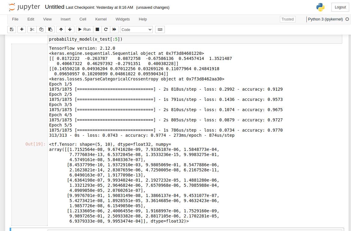
output from completed tutorial

Coming back to it

I’m going to stick with this tutorial and break it down into much smaller posts that are better detailed. I’ll update this post with links to other posts that describe specific parts of what’s going on here.

I knew this would be a large amount to learn but I didn’t predict it would be this intense to understand what’s going on there. I was sorely mistaken. I can’t even tell how much knowledge I’m missing at this point to be able to work with this, it’s so much.

Conclusion

Simply setting up the most basic model and seeing it run is very easy. Understanding what the tutorial is actually doing under the covers requires a lot of additional knowledge that I do not have. I’m looking at the output of this thing and I do not understand what I’m looking at.

This will take months or potentially years of study for me to be able to properly comprehend. But that’s OK, that’s exciting that there is so much I don’t yet know, and it’s a lot of writing for me to do as well. Loads of topics to cover!